By the Numbers

An MBS market leveraged on housing

Brian Landy, CFA | September 23, 2022

This document is intended for institutional investors and is not subject to all of the independence and disclosure standards applicable to debt research reports prepared for retail investors.

The importance of housing for valuing MBS may never have been higher than it is today. Most outstanding MBS currently trade below par, with some near the deepest discounts in market history. Nuances in housing turnover and in resulting prepayments will get magnified into differences in MBS value. Homeowner decisions to take out some of the extraordinary equity built up in recent years also should have outsized effects. Then there’s the influence of home prices on MBS loan size, net supply and, of course, credit. Despite a housing slowdown, the immediate outlook for turnover looks better than for housing overall. As for pricing, it looks like the market is in for a couple of flat years with big variation across local markets.

Outlook for turnover

Housing turnover is slowing in response to higher mortgage rates, high home prices, and concerns about the economy. Total home sales are currently about 15% below the 2019 level, when housing turnover was roughly 7 CPR. This suggests that turnover has fallen to about 6 CPR. This number is an annual average, so actual turnover could be as much as 30% lower during the winter trough and up to 25% higher during the summer peak. That suggests speeds could vary from 5.0 CPR to 8.7 CPR throughout the year.

But over a somewhat longer horizon, turnover will likely work back up to 6.5 or 7.0 CPR. The pandemic and low interest rates probably pulled forward some purchases. But many people face unavoidable reasons to move—job changes, job loss, marriage, death, having kids, and aging. Borrowers with a lot of equity can make a larger down payment to compensate for lower affordability. It is newer borrowers facing tepid HPA that could be stuck in their homes for a long time. The home purchase decision is one of many that households face. The cost of financing is one aspect of that, but not the sole aspect.

For example, the number of fixed rate purchase loans originated in June 2022 was almost the same as in June 2019, despite greater lock-in this year. So far, the Fannie Mae and Freddie Mac have pooled roughly 197,000 30-year fixed-rate purchase loans originated in June 2022. Those loans had an average loan size of $333,000 and an average note rate of 5.33%. In June 2019, the GSEs pooled 202,000 purchase loans averaging $257,000 loan size and 4.30% note rate. People need homes, in many cases regardless of the financing rate.

Cash-out refinance volumes have fallen since the start of the year but have not vanished. For example, rate-and-term refinance volume fell 86% from January through June and is likely even lower in July and beyond. But cash-out refinance volume fell only 64% over that time. And comparing June 2022 to June 2019 shows that a similar number of cash-outs—46,000—were originated in each month, despite a 5.45% note rate on the June 2022 production compared to a 4.54% note rate on the June 2019 production. Some people need the cash.

It is notable that credit scores for cash-out refinances have fallen since the start of the year. The average cash-out credit score was 736 in June 2019, 737 in January 2022, but only 719 in June 2022. This illustrates that lower credit borrowers may find a cash-out refinance is the best or even the only source of cash. Higher credit borrowers may have extracted cash opportunistically while rates were at historic lows or are more likely to have access to HELOCs and second liens to tap home equity without prepaying a first lien with an attractive rate.

Seasoned loans with the most equity should provide faster turnover and cash-out volumes than new production that is likely to face stagnating home prices. However, beware buying pools that are priced assuming optimal prepayment speeds, because turnover for those loans does not have much room to move faster. Low credit borrowers typically turnover faster, plus are more likely to use a cash-out refinance, so may be another source of value. And in a downturn an agency investor might benefit from faster defaults.

Net supply has fallen along with home sales this year. However, unless there is a broad drop in home prices supply should stay much higher than before the pandemic. Back then $20 billion a month was a roughly normal level for supply; going forward the new normal is likely to be around $40 billion a month.

Outlook for home prices

Many home price forecasts have been adjusted slower in response to higher interest rates and a potentially slowing economy. Recent home price data suggests that appreciation is falling alongside the drop in home sales. Moody’s forecast now anticipates national home price appreciation to slow over the next 12 months and, by mid-2023, be roughly flat (Exhibit 1). Their forecast holds HPA at about 0.5% until 2026, after which it slowly ramps up to around 4.5%.

Exhibit 1: There is a lot of geographic variation in home price growth

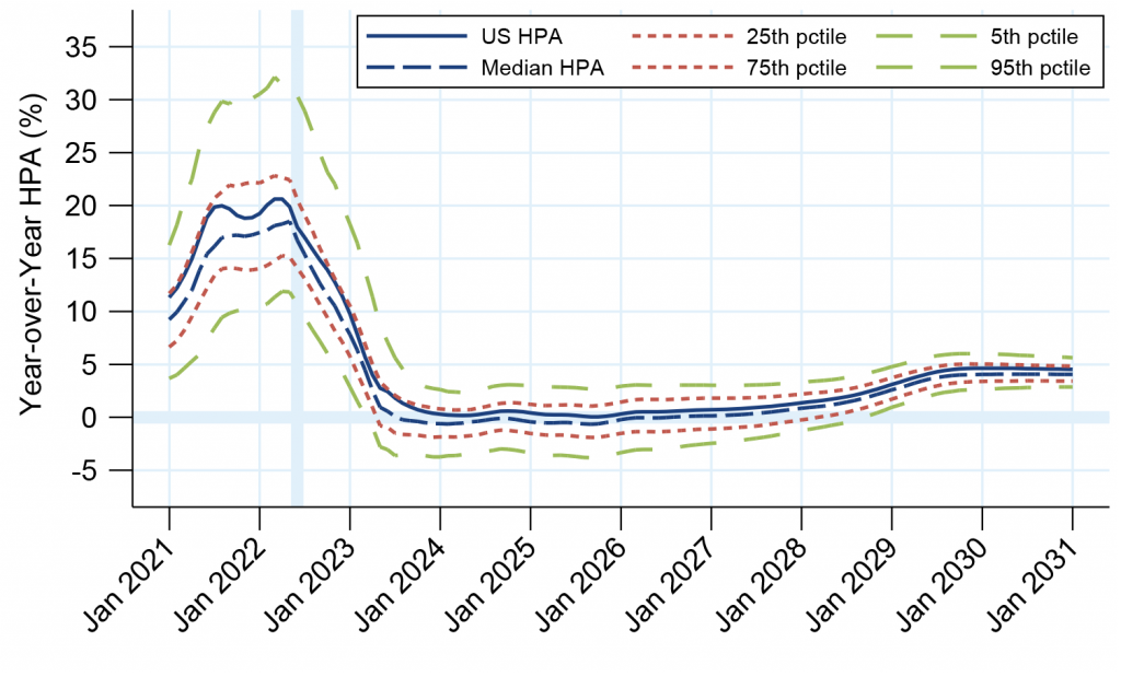
Moody’s September 2022 forecast, which starts in July 2022. CoreLogic historical home prices through June 2022. Distribution calculated using CBSA-level home prices.
Source: Moody’s, CoreLogic, Amherst Pierpont Securities

But home prices in a lot of areas do not track the national average. Many local factors influence the supply of and demand for housing. Restrictive zoning laws and lack of available land can lower supply and push prices higher. And locations can experience in- and out-migration as people look for better job opportunities or quality of life.

For example, in 2022 some locations experienced over 30% growth compared to the same month in 2021. But other locations experienced only 10% growth, while the national average peaked at around 20%. And home prices in the median location grew somewhat slower than the national average. The fastest growing states were places Idaho (37% YoY HPA), Arizona (32% YoY HPA), and Florida (30% YoY HPA). The warm climates of Florida and Arizona attracted many residents that were able to work remotely. Many Californians left for Idaho and Arizona. And Florida has no state-level income tax and was able to re-open more quickly during the pandemic.

On the other hand, home prices only grew at a peak of around 23% in California, despite the weather advantage. New York peaked at 17% in 2021, lower than the national average. Both states experienced net out-migrations and home prices suffered.

Going forward, Moody’s expects roughly half of the country to experience home price depreciation for an extended time—five years or more. Seasoned borrowers with a lot of accumulated HPA should be well positioned to weather a downturn. But people that bought homes at the peak do not have an equity cushion and could pose a credit risk in an economic downturn. This could be especially true of FHA loans and GSE loan programs that only require small down payments. Investors in private-label and credit-risk transfer securities should be especially cautious about 2022 production and watch out for regional depreciation.

Therefore, in a strong economy some potential agency supply may be captured by non-agency financing, and agency prepayment speeds might increase. And the opposite would be true in a weak economy—agency supply might increase as private label issuance shuts down, and agency prepayment speeds decrease for loans that no longer have better execution in PLS.

The backstory: linking housing to MBS

Any borrower that moves needs to pay off their existing mortgage. That creates a prepayment, regardless of whether they buy an existing or new home. And there is another prepayment if the existing home is mortgaged. Therefore, prepayments from housing turnover are closely linked to the pace of existing and new home sales. Of course, not all homes are mortgaged, or the mortgage could be financed by a private-label securitization or held on a bank’s balance sheet. So not every sale becomes an agency MBS prepayment. But the agency market is so large that it follows broad market trends.

Home sales also drive MBS supply. The balance of any new homes that are financed with agency MBS add directly to the net supply of agency MBS. Existing home sales can also contribute to net supply. If home prices are growing and existing loans are amortizing, then new loans are typically larger than the loan that is being paid off. Rate/term refinance transactions generally do not contribute to net supply since the new loan is typically replacing an existing loan with the same balance.

Home price appreciation also contributes to faster prepayments. Many borrowers rely on the equity gains from higher home values for the down payment on a new home. The borrower’s leverage means the equity position grows faster than the home’s value, enabling borrowers to buy bigger homes even though the whole market is pricing higher. However, rapid home price appreciation can lock out new borrowers that face the twin hurdles of larger monthly payments and larger down payments. And, rather than move, some borrowers may choose to extract home equity using a cash-out refinance.

Credit concerns are diminished when home price appreciation is strong. Borrowers with home equity are unlikely to allow their home to proceed to foreclosure and liquidation. A home sale is much more likely, and strong home price growth typically means there is a lot of demand to buy homes. But when home prices are weak, or if they depreciate, borrowers are more likely to default. Even borrowers that want to avoid defaulting may find it harder to sell their home if they have little equity and the housing market is weak.

History of housing turnover

The pace of housing turnover has varied greatly over the last 20 years (Exhibit 2). Two different approaches are used to estimate the prepayment speed from turnover. The first compares the pace of total home sales to the size of the current supply of single-family homes. The second approach uses data from the Census’ American Community Survey, which asks homeowners whether they lived at the same address one year earlier. Using two approaches, neither of which is perfect, allows comparison and assessment of the similarities and differences. And both offer advantages compared to estimates using discount MBS prepayment speeds, for which the data is limited and cannot measure the turnover speeds of loans that are in-the-money to refinance.

Exhibit 2: The highs and lows of housing turnover

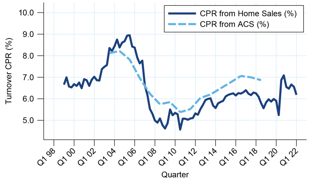
The home sales data is seasonally adjusted and the ACS data only reports moves annually, so the seasonal component of turnover is not shown.
Source: US Census Bureau American Community Survey, NAR, Amherst Pierpont Securities

Housing turnover was roughly 6.5 CPR to 7.0 CPR in the late 1990s and early 2000s. But the housing market soon took off, fueled in part by changes to the capital gains tax in 1998. Housing turnover peaked at roughly 9 CPR during this boom. The ACS estimate is a little lower than the home sales estimate, likely because the ACS methodology misses multiple sales within a year, and home flipping was popular.

Turnover plummeted to roughly 5 CPR during the financial crisis in 2008. The ACS data also fell, although not as much as the speeds from home sales. The difference is likely due to the increase in foreclosures, which could have resulted in some moves without an associated sale. Both metrics grew slowly as the housing market started its recovery in 2012. The ACS estimate stayed persistently higher than the home sales estimate, which can be attributed to the growth of the single-family rental market. Therefore, the ACS estimate is likely the better proxy for turnover in agency MBS and suggests turnover reached 7 CPR before the pandemic. The ACS data is not available during the pandemic, but home sales indicate that speeds jumped by 1 CPR, so overall housing turnover probably reached 8 CPR during the pandemic.

The net supply of agency MBS tracked the rise and fall of turnover over the last 20 years (Exhibit 3). The supply numbers tend to be noisier since a loan that pays off one month might not be re-pooled during the same month. But the correlation to turnover levels is evident. Net supply peaked during the mid-2000s and again during COVID, just like turnover. And supply was its lowest following the 2008 financial crisis. Supply even turned negative for a time, a consequence of large delinquent loan buyouts from MBS pools, before recovering alongside turnover starting in 2012.

Exhibit 3: MBS supply tracks turnover levels

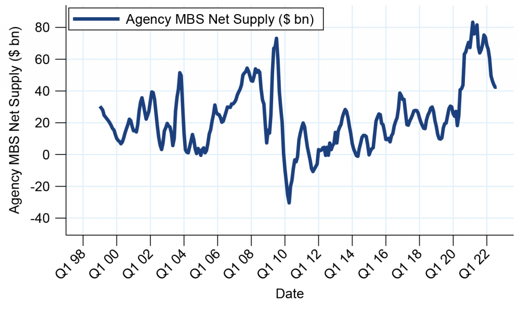
Net supply smoothed using a centered 5-month moving average.
Source: Fannie Mae, Freddie Mac, Ginnie Mae, Amherst Pierpont Securities

Interestingly, net supply peaked higher during the pandemic than it did during the housing boom, even though turnover was lower during the pandemic. The explanation is home prices, which were much larger during the pandemic than during them mid-2000s. Each new home sold was much larger and contributed more to net supply than a home sold in the prior decade. And each existing home sale contributed more to net supply since the size difference between the typical new loan and typical paid off loan was also wider. Net supply averaged roughly $20 billion/month over the few years before the pandemic but is likely to average around $40 billion/month unless home values or home sales crash.

History of home prices

The housing market has experienced significant ups and downs over the last 20 years. General wisdom has been that home prices should increase roughly 3% to 5% annually in a typical environment, but appreciation has often diverged from that level (Exhibit 4). The strong housing market in the early-to-mid 2000s was characterized by strong home price growth, which topped 10% in 2004 and 2005 according to the FHFA’s purchase-only home price index.

Exhibit 4: Strong home prices lower mortgage credit risk

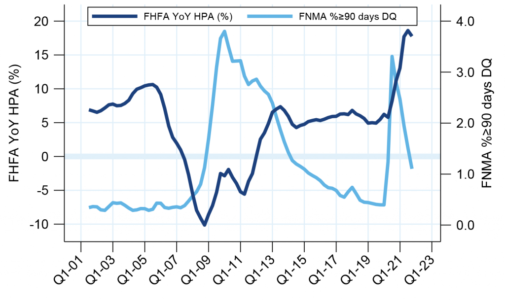
FHFA Home Price Appreciation is percentage change from one year earlier using the FHFA’s purchase-only home price index. Delinquencies from Fannie Mae’s single-family loan performance data.
Source: FHFA, Fannie Mae, Amherst Pierpont Securities

But home price growth started to slow in 2006 and homes eventually started to lose value in 2007. Many borrowers had purchased at the peak and depreciation quickly eroded the little equity they had in their homes, even pushing some underwater. The economy entered a severe recession in 2008 and pushed a lot of loans into serious delinquency. It proved difficult for borrowers with little-to-no equity to recover. Borrowers and lenders needed to accept short sales, or foreclose on the home, or pursue loan modifications that attempted to lower payments.

The pace of recovery quickened after home price appreciation turned positive in 2012. But delinquency rates never quite recovered to the pre-crisis level.

Borrowers with equity and in a strong housing market can often sell the home to avoid a default. Perhaps they are delinquent for a few months while marketing the home and waiting for a sale to close. This played out during the pandemic. Delinquency rates skyrocketed at the start of the pandemic when the economy shut down and many people found themselves unemployed. But a lot of people kept their jobs and started to work from home, while their kids attended school from home. People moved to bigger homes in nicer locations, boosting demand for housing. But the supply of housing was tight, so demand caused a record increase in home prices. As the economy reopened, this contributed to fast curing of many delinquencies, especially in comparison to the post-crisis era.

Home prices, particularly borrower equity, is therefore very important for bonds exposed to credit risk, like private-label securitizations and credit-risk transfer deals. This is less impactful to investors in agency MBS, since the credit risk is guaranteed by Fannie Mae, Freddie Mac, or a government agency. Although delinquencies and defaults can influence prepayment speeds, and bond values.

Home price appreciation also influences net supply. More expensive homes need larger mortgages. If those are new homes, the larger balance adds directly to net supply. But if those are existing homes, HPA increases the balance difference between the new loan used to buy a home and the old loan that is paid off. That difference also contributes to net supply.

Home price appreciation also allows borrowers to do cash-out refinances, which lift supply and prepayment speeds. However, borrowers are less likely to do a cash-out when interest rates are high, and lenders turn their focus to second liens and HELOCs. But some borrowers may not qualify for a second lien or HELOC, leaving a cash-out refinance as the only option to get equity to pay for things like education.